Introduction
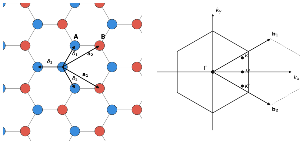
Given the above coordinate choice for graphene unit cell, the band structure of a (N,0) CNT (Zig-Zag CNT), obtained from the tight-binding model of graphene (Castro Neto et al. 2009), is expressed as (Obtained by putting the quantization condition \(N a k_y = 2\pi m\) in the graphene band structure):
\[\begin{equation} \label{eq:band-structure} E = \pm t_0 \sqrt{f(k_x, m)} = \pm t_0 \sqrt{1+4\cos\bigg{(}\frac{3k_xa}{2}\bigg{)}\cos\bigg{(}\frac{\pi m}{N}\bigg{)}+4\cos^2\bigg{(}\frac{\pi m}{N}\bigg{)} } \end{equation}\]
where \(t_0 = 2.5eV\) is the tight-binding coupling constant, where \(a\) is the lattice constant and m is an index that runs from \(0\) to \(N-1\). A thorough derivation can be found in (Schönenberger 2015), although with axes rotated.
Analytical expression for band-gap
CNT is one of those nice systems where the band-gap can be expressed analytically. In \(\eqref{eq:band-structure}\), consider the bands with a \(+\) sign. Then the band-minimum, \(E_{min_m}\) for a given band index, \(m\), occurs when \[\begin{equation} \partial_{k_x}f(k_x, m)=0 \implies \frac{3k_xa}{2} \in \{0,\pi\} \end{equation}\]
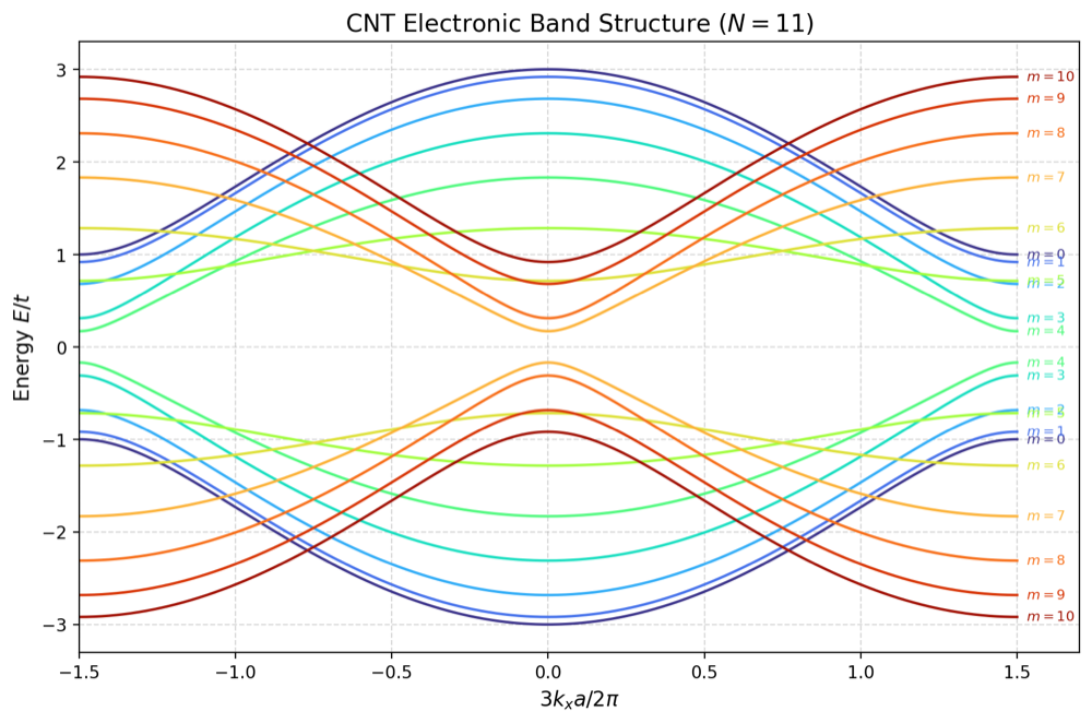
while the minimum of the set \(E_{min_m}\) across all bands, as \(m\) is varied is obtained when the quadratic equation in \(\cos(\frac{\pi m}{N})\) is minimized: \[\begin{equation} \begin{split} \partial_{\cos(\pi m/N)}f(k_x, m)\bigg|_{\frac{3k_xa}{2} \in \{0,\pi\}} &= 0 \\ \implies \cos\bigg(\frac{\pi m}{N}\bigg) &= -\frac{1}{2}\cos\bigg(\frac{3k_xa}{2}\bigg)\bigg|_{\frac{3k_xa}{2} \in \{0,\pi\}} \\ &= \pm \frac{1}{2} \end{split} \end{equation}\] which means \(\cos\bigg(\frac{\pi m}{N}\bigg)\) needs to be as close to \(\pm\frac{1}{2}\) as possible. This is exactly possible whenever \(N = 3m\), then band-gap is exactly 0 and we call such a CNT metallic. Though in this article, we will consider only CNTs with a bandgap so let us restrict ourselves to when \(N=3m-1\), i.e \(N=8, 11, 14, 17\) etc. A representative band-diagram is shown for \(N=11\) below:
Given a value of \(N\), \(m\) will take values in the set \(\{0, 1, 2, \ldots, N-1\}\). Let \[m_0 := \operatorname*{arg\,min}_{m} \left\{\left| m - \frac{N}{3} \right|, \left| m - \frac{2N}{3} \right|\right\}.\] The band-minima is then written as (pairing the value of \(m_0\) with \(\frac{3k_x a}{2} = \pi /0\)): \[\begin{equation} \label{eq:bandgap} E_g = 2t_0\sqrt{1-4\cos\bigg{(}\frac{\pi m_0}{N}\bigg{)}+4\cos^2\bigg{(}\frac{\pi m_0}{N}\bigg{)} } . \end{equation}\]
Analytial expression for Density of States
Good point to obtain an expression for the density of states near the band-minimum. First, we need to show the following approximation holds near the band-minimum:
\[\begin{equation} \label{eq:dkx-dE} \frac{d}{dE} \bigg{(}\frac{3k_x a}{2}\bigg{)} \approx \frac{|E|}{t_0\sqrt{E^2-(E_g/2)^2}} \end{equation}\]
In section 1.1 we discovered that a neighbourhood of band minimum comprises of \(m_0\) with \(\frac{3k_x a}{2} \approx \pi\). So equation \(\eqref{eq:band-structure}\) around band-minimum can be rewritten as a taylor expansion around \(\frac{3k_x a}{2} = \pi\): (Hereafter, \(k_x\) refers to the small-signal expansion around \(k_x = \frac{2\pi}{3a}\)) \[\begin{equation} E \approx \pm t_0 \sqrt{1+4\cos\bigg{(}\frac{\pi m_0}{N}\bigg{)}\bigg{(}-1-\frac{1}{2}\bigg{(}\frac{3k_xa}{2}\bigg{)}^2\bigg{)}+4\cos^2\bigg{(}\frac{\pi m_0}{N}\bigg{)} } \end{equation}\] Plugging in the value of \(E_g\) from \(\eqref{eq:bandgap}\), we get:
\[\begin{equation} E \approx \pm t_0 \sqrt{\bigg{(}\frac{E_g}{2t_0}\bigg{)}^2-\bigg{(}2\cos\bigg{(}\frac{\pi m_0}{N}\bigg{)}\bigg{)}\bigg{(}\frac{3k_xa}{2}\bigg{)}^2 } \end{equation}\]
Since \(m_0\) takes \(\cos(\frac{\pi m_0}{N})\) to be as close to \(\frac{1}{2}\) as possible, for a big enough N, we can approximate the above equation as:
\[\begin{equation} E \approx \pm t_0 \sqrt{\bigg{(}\frac{E_g}{2t_0}\bigg{)}^2-\bigg{(}\frac{3k_xa}{2}\bigg{)}^2 } \end{equation}\] Rerrangment gives:
\[\begin{equation} \label{eq:kx-of-E} \frac{3k_xa}{2} \approx \pm \frac{1}{t_0}\sqrt{E^2 - \bigg{(}\frac{E_g}{2}\bigg{)}^2} \end{equation}\]
\(\eqref{eq:dkx-dE}\) follows from differentiating \(\eqref{eq:kx-of-E}\) with respect to \(E\).
From here, the calculation of density of states is straightforward. Density of States is defined as:
\[\begin{equation} D(E) = \frac{1}{L}\frac{ \text{\# States in [E, E+ dE]}}{dE} \end{equation}\]
For a periodic system, this means counting the number of values of \(k_x\) whose energy lies in the range \([E, E+dE]\) i.e. \(dk(E)\). We already know \(dk(E)\) from \(\eqref{eq:dkx-dE}\).
k-states are spaced uniformly with space \[\begin{equation} \label{eq:k-spacing} d \bigg{(}\frac{3k_x a}{2}\bigg{)} = \frac{3\pi a}{L} \end{equation}\]
Now we compute \(D(E)\) in steps, first we find the numerator ie # states in [k, k+dk]: \[\begin{equation} dk(E) = \frac{d}{dE} \bigg{(}\frac{3k_x a}{2}dE \bigg{)} \approx \frac{|E|dE}{t_0\sqrt{E^2-(E_g/2)^2}} \end{equation}\]
The number of states in this range of \(dk\) is given by dividing above equation by \(\eqref{eq:k-spacing}\) \[\begin{equation} \frac{1}{ \frac{3\pi a}{L}}\frac{d}{dE} \bigg{(}\frac{3k_x a}{2}dE \bigg{)} \approx \frac{1}{ \frac{3\pi a}{L}}\frac{|E|dE}{t_0\sqrt{E^2-(E_g/2)^2}} \end{equation}\] Dividing by L gives: \[\begin{equation} D(E) \approx \frac{1}{3\pi a}\frac{|E|}{t_0\sqrt{E^2-(E_g/2)^2}} \end{equation}\]
Degeneracy
But the equation above is not yet correct, since there is an eight-fold (\(2 \times 2 \times 2\)) degeneracy in a CNT:
In \(\eqref{eq:band-structure}\), \((k_x, m)\) and \((-k_x, N-m)\) give the same energy (a factor of \(2\)).
Electron spin takes two values (a factor of \(2\)).
Each band is symmetric about its minimum, and our expression considered only a single branch of the expansion around the band-minimum (a factor of \(2\)).
The last degeneracy can also be seen in the figure 2 in Introduction section. The final Density of States is then given as: \[\begin{equation} D(E) \approx \frac{8}{3\pi a}\frac{|E|}{t_0\sqrt{E^2-(E_g/2)^2}} \end{equation}\]
Verification
Let us derive the surface charge density expression Each state has its charge distributed uniformly across the cylinder. So that the surface charge density is given as (remember DoS is already per unit length, so we just need to divide by the circumference of the cylinder while computing surface charge density): \[\begin{equation} \sigma = \frac{q}{2\pi R}\int_{E_1}^{E_2} D(E)f(E)dE \end{equation}\]
\[\begin{equation} \sigma = \int_{E_1}^{E_2} \frac{8q}{6\pi^2 R a}\frac{|E|}{t_0\sqrt{E^2-(E_g/2)^2}}f(E)dE \end{equation}\] From geometry, we know the relation: \[\begin{equation} 2R\sin\frac{\pi}{N} = \sqrt{3}a \end{equation}\] For big enough N, we can linearize sin function and this gives: \[\begin{equation} \sigma = \int_{E_1}^{E_2} \frac{8q}{3\sqrt{3}\pi a^2 N}\frac{|E|}{t_0\sqrt{E^2-(E_g/2)^2}}f(E)dE \end{equation}\] This agrees with the expression we have in Eq. 15 of (Leonard and Stewart 2006)